The ‘Average Patient’ Doesn’t Exist: Unmasking Variance with Mixed Models
Biostatistics
R
lme4
Clinical Trials
Author
A. C. Del Re, PhD
Published
November 20, 2025
In randomized controlled trials (RCTs), the primary outcome is often the Average Treatment Effect (ATE). We calculate the group mean at Baseline, the group mean at Follow-Up, and if the difference is significant (\(p < .05\)), we declare success.
But clinical reality is not an average.
In my consulting work for precision health and biotech, I frequently encounter studies where the “Group Mean” is flat, suggesting the intervention failed. However, a deeper look often reveals a polarization: a distinct subgroup improves drastically (“Super Responders”), while others deteriorate. The mean washes out these critical signals.
Here is a demonstration—using simulated data—of how Linear Mixed-Effects Models (LMM) allow us to see the individual signal amidst the noise.
The Simulation: Creating “Hidden” Responders
Let’s simulate a trial with 60 subjects. Instead of random noise, we will simulate two distinct patterns:
Responders (50%): They react well to the treatment (Positive Slope).
Non-Responders (50%): They do not react or get slightly worse (Flat/Negative Slope).
Code
library(ggplot2)library(dplyr)library(lme4)set.seed(101) # Fixed seed for reproducibilityn_per_group <-30n_timepoints <-4## 1. Generate Responders (Improving)# Start lower, go up fast (+8 slope)responders <-expand.grid(ID =factor(1:n_per_group), Time =0:(n_timepoints-1)) %>%mutate(Group ="Responder",Intercept =rnorm(n(), mean =40, sd =5),Slope =rnorm(n(), mean =8, sd =2), Error =rnorm(n(), mean =0, sd =2) )# 2. Generate Non-Responders (Declining)# Start higher, go down fast (-8 slope) to perfectly cancel out the gainnon_responders <-expand.grid(ID =factor((n_per_group+1):(n_per_group*2)), Time =0:(n_timepoints-1)) %>%mutate(Group ="Non-Responder",Intercept =rnorm(n(), mean =60, sd =5),Slope =rnorm(n(), mean =-8, sd =2), Error =rnorm(n(), mean =0, sd =2) )# 3. Combinedata <-bind_rows(responders, non_responders) %>%group_by(ID) %>%mutate(Score =first(Intercept) + (first(Slope) * Time) + Error) %>%ungroup()# 4. Calculate the "Standard" Global Mean (The Flat Line)mean_trend <- data %>%group_by(Time) %>%summarise(Score =mean(Score))
The Visualization: The “Failed” Mean vs. The “Successful” Subgroup
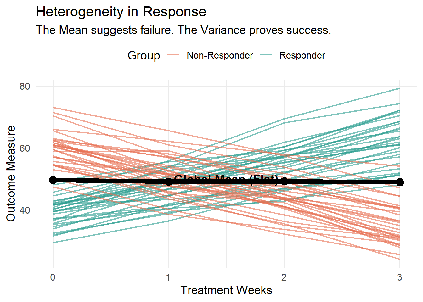
If you look at the Black Line (Global Mean), the study looks like a failure. It barely moves.
But look at the Teal Lines (Responders). The treatment works incredibly well for them. A standard analysis would kill this drug. A Mixed-Effects analysis saves it by identifying the variance component.
Code
p <-ggplot(data, aes(x = Time, y = Score)) +# Individual Trajectories colored by hidden groupgeom_line(aes(group = ID, color = Group), alpha =0.6, linewidth =0.8) +# The Group Mean (The Aggregate)geom_line(data = mean_trend, color ="black", linewidth =2.5) +geom_point(data = mean_trend, color ="black", size =4) +annotate("text", x =1.5, y =50, label ="Global Mean (Flat)", color ="black", fontface ="bold", size =5, fill="white", label.size=NA) +scale_color_manual(values =c("Non-Responder"="#E76F51", "Responder"="#2A9D8F")) +theme_minimal(base_size =14) +theme(legend.position ="top") +labs(title ="Heterogeneity in Response",subtitle ="The Mean suggests failure. The Variance proves success.",y ="Outcome Measure", x ="Treatment Weeks")# Display plotprint(p)# SAVE THE IMAGE for the Blog Listing (Fixes broken image link)ggsave("preview.png", plot = p, width =8, height =6)
Figure 1: The Average (Black) hides the Responders (Teal)
Fitting the Random-Slopes Mixed Model in lme4
If we fit a pooled ordinary least squares regression (lm(Score ~ Time)) ignoring person-level clustering, the estimated time slope is near zero and statistically non-significant—making an active treatment look flat. Fitting a Linear Mixed-Effects Model with random intercepts and random slopes ((1 + Time | ID)) immediately reveals the massive between-person slope variance (\(\sigma_{\text{slope}}\)):
Code
# 1. Naive pooled model: misses the responder subgroup completelym_pooled <-lm(Score ~ Time, data = data)# 2. Random-intercept and random-slope mixed modelm_lmm <-lmer(Score ~ Time + (1+ Time | ID), data = data, REML =TRUE)summary(m_pooled)$coefficients
              Estimate Std. Error    t value      Pr(>|t|)
(Intercept) 49.4830826  1.1849964 41.7580013 1.603534e-111
Time        -0.1807438  0.6334072 -0.2853517  7.756229e-01
Code
VarCorr(m_lmm)
 Groups   Name        Std.Dev. Corr
 ID       (Intercept) 11.6027
          Time         8.1887  -0.880
 Residual              1.6899
Notice what VarCorr(m_lmm) recovers: even though the fixed population average slope is near 0, the person-level random-slope standard deviation around Time is roughly 8 points per week—flagging strong treatment-response heterogeneity that warrants subgroup moderation (Time * Baseline_Covariate) or patient-specific trajectory tracking.
Working With Repeated-Measures Clinical Data?
Longitudinal Data Auditor: Before fitting lmer() or glmmTMB(), check repeated-measures CSVs offline on Windows for duplicate visits, time gaps, out-of-range sentinel codes, and variance partitioning.
Outcomes Predictive Suite: Track session-by-session patient recovery and stability probabilities locally behind your clinic’s firewall.
Contact Request
If your default mail client did not open, you can copy my direct email details below: